Calibration

The calibration view allows the user to check whether the measurement setup is properly aligned, whether the sample is in focus of the camera, specify calibration parameters, and perform reference measurements.

View

By default the calibration view will show a live view of the the raw data returned by the instrument.

For HSI cameras this will consist of a 2D image that represents a physical 1D line. One of the directions of the image (x or y, typically y) represents the spectral direction of the data. This moving along that direction will choose the same spatial pixel, but at a different spectral wavelength. The other direction is the spatial direction. Moving along that direction will look at different spatial pixels, but for the same wavelength.

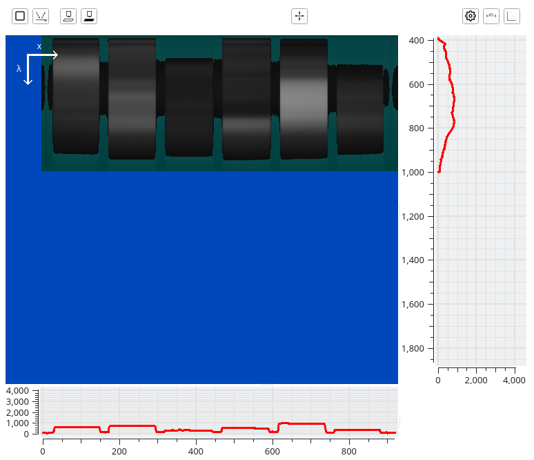
The view features axis drawn in white color that show the orientation of the spatial and spectral axes:

The data is displayed with a grayscale color map. Darker pixels indicate lower counts, lighter pixels indicate higher counts.

The exception are the lowest and highest 5 percent of the value range of the device:

• For pixels that are within 5 percent of the lowest value (typically 0) of the value range, their grayscale (near black) pixels will be overlayed with a teal color.

• For pixels that are within 5 percent of the highest value of the value range, their grayscale (near white) pixels will be overlayed with a pink color.

• Pixels that have exactly the lowest value of the range (typically 0) will be colored in a dark blue distinct from the dark blue background of the view itself.

• Pixels that have exactly the highest value of the range, indicating saturation, will be colored in red.

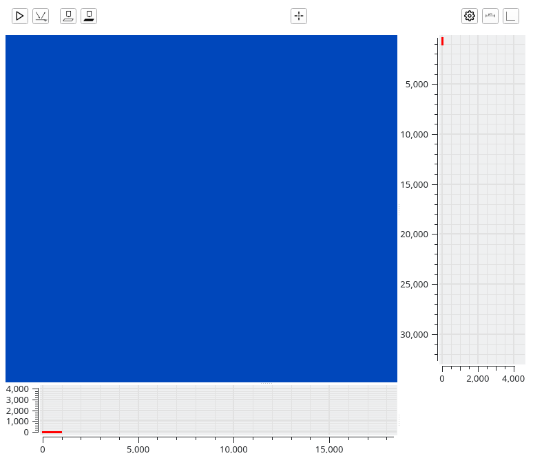
The following image shows a gradient map that demonstrates this:

The background of the image is the background blue of the calibration view. On the left and right sides there are rectangles of solid dark blue (distinct from the background) and red to demonstrate the color of pixels if they have the lowest value (typically zero) or the highest value (saturated). In the middle there is a gradient where at the ends the teal/pink overlays are applied in the same manner as they are with the pixels in the calibration view.

Completely saturated pixels should always be avoided, because it cannot be determined whether the amount of light was just enough to reach that numerical value, or was already beyond it. This can lead to numerical artifacts.

Average Views

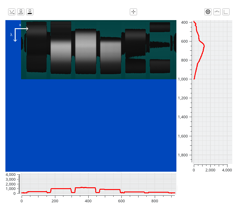
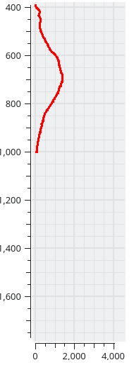
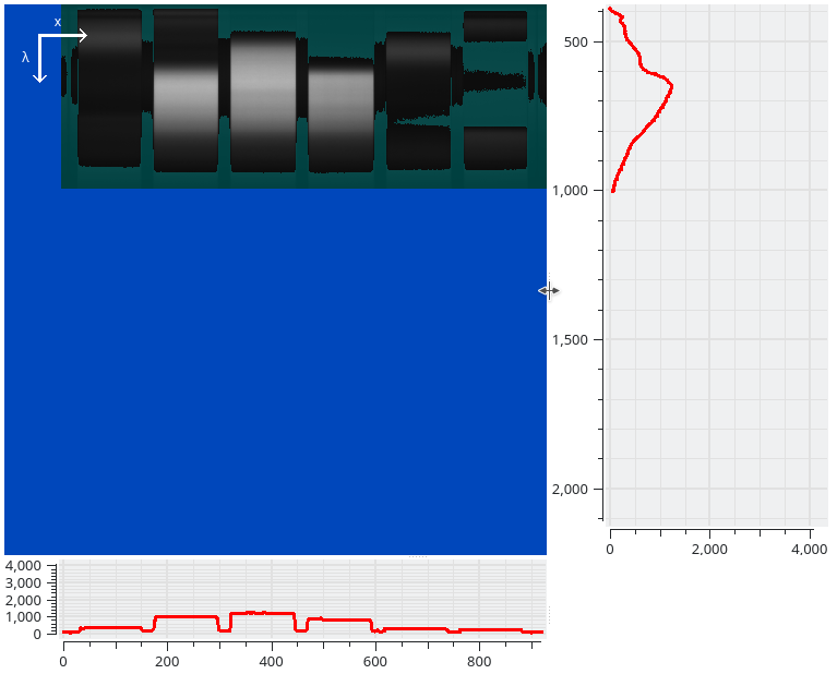
Towards the right hand and the bottom there are two views that show the average spectrum of the given pixels along both axes. On the right the view averages all columns and displays it as a plot:

On the bottom the view averages all rows:

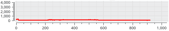
The axes of the plots are as follows: for the plot on the right the axis on the left side of the plot is the abscissa of the plot, and the axis on the bottom side of the plot is the ordinate. (The plot’s axes are rotated to match what part of the image are averaged.) The plot at the bottom follows the more standard layout of the bottom axis being the abscissa and the left axis being the ordinate.

The abscissa of the plots will either be a pixel index (0 for the first pixel, 1 for the second, etc.) if that axis of the index is the spatial axis, or the wavelength of the spectral band in nanometers.

The ordinate of the plot will always be the value range of the camera.

The abscissa of the bottom plot is a pixel index in our case, starting at 0, and ending at the size of the sensor (minus one). The abscissa of the right plot is the starts at 391.138 nm and ends at 1000.515 nm, which is the wavelength range of the HSI sensor.

The ordinate of both plots ranges from 0 to 4095, which is typical for a sensor with 12 bits of precision.

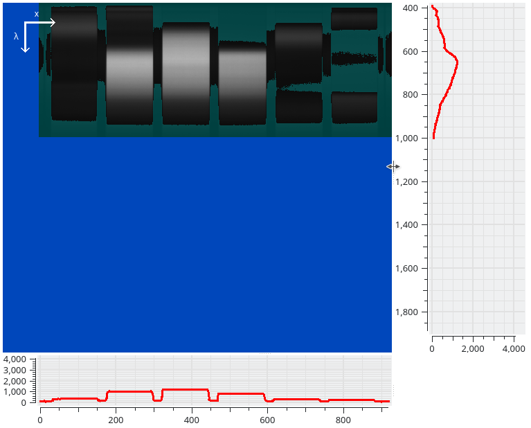
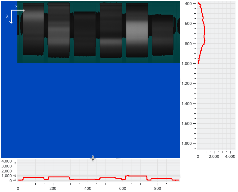
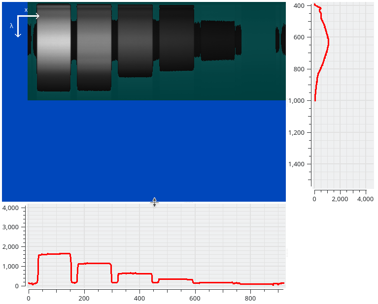
The relative sizes of the average views and the image view can be updated by dragging the splitters between the image view and the plots while the left mouse button is pressed:

Individual Row and Column Selection

The charts at the right and the bottom of the window can also display the values of a selected row and column, in addition to the averages they always show.

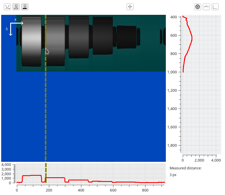
For this click in the image view with the left mouse button once. A cross-hair will immediately appear, and an additional curve is plotted in the chart views directly underneath the mouse pointer:

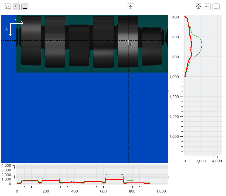
The plot to the right will show the intensity of the column underneath the mouse (along the vertical crosshair line). The plot on the bottom will show the intensity of the row underneath the mouse (along the horizontal crosshair line).

Click on the image view again to lock in the current position. The charts to the right and the bottom will still be updated, but the positions at which they are taken will remain.

Click on the image view a third time will drop the crosshair and revert to the original view.

Spatial Distance Measurement

It is also possible to measure the amount of pixels between two rows or columns in the image. For this click in the image view with the right mouse button once where to start the measurement:

A line will be drawn in the image at the position the mouse was clicked with the right mouse button. In this case the line will be vertical because the spatial of direction is horizontal. If the spatial direction were vertical in the camera raw frame, the line would be horizontal instead.

A second line will follow the mouse around when the cursor is moved. Clicking with the right mouse button a second time in the view will lock the line in.

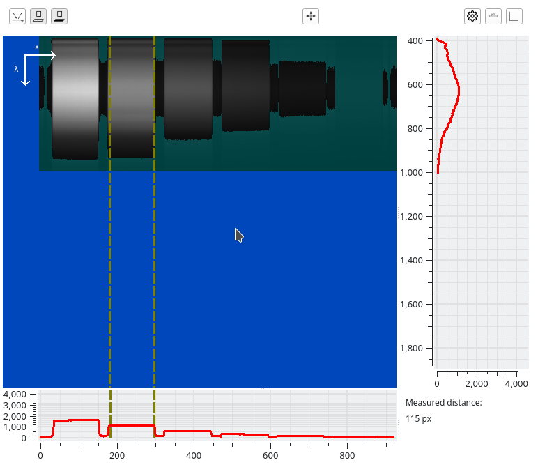
The bottom right corner will show the amount of pixels that have been measured between both lines.

Click in the image with the right mouse button a third time to revert to the original view without the distance measurement.

If the measured distance is locked in, it can be used to automatically caclulate the pixel size when configuring the calibration settings, see below for details.

Note

The spatial distance measurement mode and the individual row and column selection modes are mutually exclusive. If one mode is activated while the other is still active, only the newly activated mode will remain active.

Mode

Above the image view there are several buttons. The first button allows the user to select the referencing mode to use for recordings. The icon of the button indicates the current referencing mode.

Clicking on the button will open a menu to allow the user to select the chosen referencing mode:

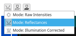
Switching between modes will not affect which references have actually been measured, it will only affect which reference buttons are shown.

Reflectances

The reflectances referencing requires a white reference measurement. (A dark reference measurement is optional.) Both the white and dark reference buttons will be shown next to the referencing mode button.

A more detailed explanation of reflectance measurements can be found in the concepts chapter.

Raw Intensities

The raw intensities referencing mode indicates that the user does not want to perform a white or illumination referencing step when recording the data.

By default no reference buttons will be shown at all in this mode.

If the device has radiometric corrections enabled, this mode will have the same icon, but a different text (either Radiances or Relative Radiances, depending on the type of corrections). In either case will the dark reference measurement button be visible. If the device’s corrections produce absolute Radiances, the user must measure a dark reference before they can record data in this mode; if the device’s corrections produce Relative Radiances, the dark reference measurement is optional.

Devices that support radiometric corrections will typically have a parameter that allows the user to switch them on or off. Changing that parameter will also change the text of this option.

Illumination Corrected

The illumination corrected referencing mode will make recordings that use an illumination reference to calibrate out spatial differences in the illumination, while not affecting the spectral response.

A more detailed explanation of illumination corrected measurements can be found in the concepts chapter.

The illumination and dark reference buttons will be shown next to the referencing mode button.

Note

The illumination reference measurement button will have the same icon as the white reference measurement button, but it is a different button.

Measuring References

Next to the referencing mode button there may be one or more buttons that allow the user to perform reference measurements. By default there are three types of buttons that may appear here:

• Measure white reference

• Measure illumination reference

• Measure dark reference

The buttons may be in two states:

• Not depressed: the reference has not yet been measured. Click the button to begin the process of measuring the reference.

• Depressed: the reference has been measured. Click the button to remove the current reference measurement from memory.

Note

How the buttons look in their depressed / not depressed state will depend on the operating system and the style selected for the operating system. They may therefore look slightly different from the buttons shown in these screenshots.

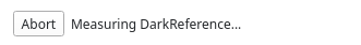
To measure a reference click on the corresponding button. The buttons will then be replaced by a text that indicates which measurement is currently being measured. The user can also click on the Abort button to abort the current reference measurement that is in progress:

To perform a reference measurement fluxTrainer will perform the following steps:

1. fluxTrainer will stop data acquisition from the camera

2. fluxTrainer will cause any light control device to enter the appropriate state for this type of reference

3. If the camera has an integrated shutter, fluxTrainer will close that shutter that if a dark reference is to be measured

4. fluxTrainer will start data acquisition from the camera again

5. fluxTrainer will acquire one or more camera frames to use as the reference measurement

6. fluxTrainer will stop data acquisition from the camera

7. fluxTrainer will cause any light control device to enter the appropriate state for normal acquisition

8. If the camera has an integrated shutter, fluxTrainer will open that shutter

9. fluxTrainer will start data acquisition again

The amount of frames that fluxTrainer will acquire to use in a reference measurement can be configured in the reference settings. When more than one frame is measured, the average of all reference frames will be used when it is applied to a HSI measurement.

Device-Specific Reference Types

Some (rare) devices may also have support for different device-specific reference types. In that case instead of the standard reference buttons, a single button will be shown that opens a menu for all available references:

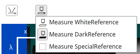
In that case clicking on the corresponding menu items is equivalent to clickin on the respective buttons in the standard case.

Motion Control Integration

If motion control devices are present, they will not influence the calibration process. The calibration logic exists independently of the motion control device integration.

The user can easily access the motion control window via the additional motion control button, , above the image view. This is useful for two situations:

• If a z-axis is connected that allows the user to manipulate the focus of the camera, the z position can be changed in the motion control window while the calibration view is open. This allows the user to verify from the camera frame whether the sample is actually in focus.

• If a y-axis is connected (or an xy-table), and there is a white reference at a specific position, the user can use the motion control window to move to that position before performing the corresponding reference measurement.

Light Control Integration

The calibration view influences light control devices. In the default acquisition mode and when measuring any reference that is not a dark reference, all connected light control devices will be set to the default Parametrized state (which typically means they are on). When measuring a dark reference they will be set to the Force Off state, instead.

See the light control chapter for further details.

Miscellaneous

On the top right part of the calibration view there are additional buttons that provide optional functionality.

Reference Settings

The settings button will open the reference settings window:

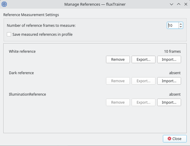
At the top the user can configure how many reference frames fluxTrainer will acquire when performing a reference measurement. This does not affect already measured references, it will only affect future reference measurements.

Below that the user can indicate with a check box to save the measured references in the profile. This will have no immediate effect. If the user proceeds to save the current settings in a profile after enabling this setting, the profile will also include the references that were measured. When connecting to such a profile, any reference measurements that were saved as part of that profile will be loaded again, and become instantly available.

It is recommended to only store references in profiles if there are no major variations in the lighting conditions and the camera sensor characteristics over time, so that a reference stored in a profile will not deviate from a reference measured at a later point in time.

In the middle of the window there is a list of references that the device supports. It will indicate how many frames are part of each reference measurement, if present.

The user can remove a reference measurement here (as if they had clicked on the corresponding button), and they can export and import reference measurements. Exported references are saved in a HDF5-based format with the file extension .fluxref.

When importing saved references the relevant camera parameters must match the parameters the reference was measured with. If that is not the case, it depends on the situation:

• If the size of the reference data differs (because the user selected a different ROI, for example), then the exported reference cannot be imported. (The user may change the parameters of the camera to match those of the reference and then import it though.)

• If the size of the reference data matches, a warning will be displayed. The user has the option to override the warning and to import the reference even if it is not compatible with the current device parameters.

Calibration Settings

Click on the calibration settings button to open the calibration settings window:

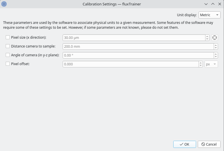
Here the user may specify various settings that describe the measurement setup. Some filters use this information to obtain more accurate results.

At the top right of the window the user can specify the measurement system they want to use to enter the quantities in. Internally all values will always be stored in metric units, but for convenience the user has the option to select different measurement systems.

There are currently four calibration settings the user may configure. The following diagram shows all four quantities in a 3d-like view:

The line that is being recorded by the camera is highlighted in light gray here.

The following diagram shows the top-down view of the system with all relevant quantities:

Finally there is also a side view:

Not all quantities may need to be set. To set a quantity, first check the checkbox before that quantity to indicate it should be present, and then enter the desired quantity on the right side of the window.

The following subsections explain the quantities:

Pixel size (x)

The size of an individual pixel in the measured sample.

The user may click on the compute size from measurement button. This will open a new window:

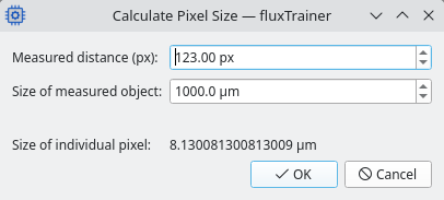
The upper edit box holds the measured distance of an object in pixels. If a spatial distance measurement was made previously, that measurement value will be filled in by default.

The lower edit box holds the size of the measured object in physical units. This must be provided by the user.

At the bottom the calculated physical size of an individual pixel will be displayed. Clicking the OK button will use that as the value for the pixel size.

Angle of camera

Describes the angle of the camera in the y-z plane. As this is a line camera the sign of the angle is not relevant, hence it should always be positive.

The camera is currently assumed to have no angle in the x-y and y-z planes.

Distance camera to sample

The distance of the camera to the sample following the line of sight of the camera.

Pixel offset

By default fluxTrainer will assume that light entering the camera at the pixel at the center of the current line is perpendicular to the sample (disregarding the y-z angle).

If that is not the case, because the user selected a ROI for example, this setting allows the user to configure the offset from the center of the current ROI at which point the light enters the camera perpendicularly. (Again disregarding the y-z angle.)

The user can select whether to specify this in pixels or in physical units.

White Reference Reflectivity

An ideal white reference reflects one hundred percent of all light, across all wavelengths. In practice that is not possible, and good white reference materials will typically reflect at least 98 percent of the light they are illuminated by.

The amount of light reflected may slightly depend on the wavelength though. It is possible that a good white reference material will reflect 98 percent of light on one end of the spectral range, and 99 percent on the other end.

In some applications this difference is not relevant. But for measurements that need a large amount of precision, knowing the reflectivity curve of the white reference material is crucial for accurate results.

fluxTrainer allows the user to provide a reflectance spectrum for the white reference material. This reflectance spectrum is used to correct the measured white reference and correct the white reference when it is being applied to be a “true” white reference measurement.

This also allows for the user to use a completely different material as a white reference, as long as the reflectance spectrum of the material is never close to zero.

Clicking on the white reference reflectivity button, a window opens where the white reference reflectivity spectrum can be provided:

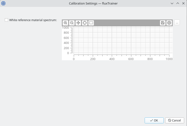
To provide such a measurement first enable the checkbox next to the White reference material spectrum label.

Then click on the … button at the right side to load a spectrum from disk. The spectrum may be specified in either CSV or JCAMP-DX formats.

Once the spectrum has been loaded the chart view will display the reflectance curve.

Closing the window with the OK button will tell fluxTrainer to remember the curve. The button for opening the white reference reflectivity window will now have also changed to to indicate that a white reference material curve has been provided by the user.

JCAMP-DX Import

The file that is opened by the user must contain only a single spectrum. If the selected file contains multiple spectra, an error will be shown.

If the JCAMP-DX is not in reflectances (because it is stored in absorbances, for example), fluxTrainer will attempt to automatically convert the spectrum to reflectances.

CSV Import

The CSV file must not have any header line. Quoted cells with a " character is supported. The separator will be automatically detected; it may either be a comma (,), a semicolon (;), or whitespace (space or tab). The decimal separator must be a period (.), and no thousands separator must be used. Scientific notation in the form 5.3e-7 is supported.

The CSV file must have exactly two columns. The first column has to contain the wavelengths in nanometers for which the spectrum is provided. The second column has to contain the reflectance values on a scale from 0 to 1.

If the CSV file has exactly two rows (but more than two columns), it will also be accepted, and the data is assumed to be transposed. (The first row being the wavelengths, the second being the corresponding reflectance values.)

The following is an example CSV file that could be imported by fluxTrainer:

400,0.98
450,0.98
500,0.99
550,0.99
600,0.99
650,0.99
700,0.99
750,0.99
800,0.99
850,0.99
900,0.98
950,0.97
1000,0.95

Wavelength Interpolation

The wavelengths of the spectrum do not need to exactly match the wavelengths of the camera. There must be sufficient overlap in the wavelength ranges. The provided reflectivity curve will be interpolated by fluxTrainer onto the wavelengths of the camera.

Manual Acquisition Mode

If the setting Automatically acquire data when instrument view is open is disabled, then an additional button is shown in the top left corner of the calibration view, and the acquisition does not automatically start:

Pressing the button will start acquisition and it changes to a stop button:

Pressing the reference measurement buttons will behave like the following:

• If the user has currently explicitly started acquisition then the reference measurement buttons will behave the same as if automatic acquisition were active: acquisition is stopped, the reference measurement occurs, and acquisition is started again.

• If the user has currently stopped acquisition, then clicking on a reference measurement button will record that reference. After that is done acquisition will be stopped again.