Concepts

Graph and Nodes

Models in fluxTrainer are designed in the form of a Graph. A graph consists of various nodes with connections between the nodes. A node may have both inputs (displayed on the left side of the node), and outputs (displayed on the right side of the node).

There are three types of node:

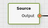
Source: the node at which data processing starts. It has exactly one output (called Output), and all input data that a model should process enters the graph through this node. At the moment graphs contain exactly one Source.

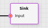
Sink: a node that takes data and interfaces it with the outside world. For example, an Output Sink may be used to extract data from a model in fluxEngine, while a Display Sink may be used to visualize the result of a model during live processing in fluxRecorder.

Filter: a node that processes data. It will have at least one input and at least one output. This type of node will perform an algorithm on the supplied input data and provide the result of that algorithm in its outputs.

Any output of a node may be connected to any number of inputs of other nodes, but an input of a node must have exactly one connection that defines where the data comes from.

Outputs of nodes may be dangling, i.e. there may be outputs of nodes that don’t have any connections. In that case the data that that node produces will not participate in further data processing in the graph.

Loops (cycles) are not allowed in the graph.

HSI Cubes

fluxTrainer works with hyperspectral data. Hyperspectral data is stored in the form of a HSI cube. A HSI cube consists 3 dimensions: the y coordinate, the x coordinate, and the wavelength. A HSI cube can be though of as an image with many colors. Each pixel of a HSI cube with coordintes (y, x) stores an individual spectrum. Internally fluxTrainer will always store cubes in the BIP (band interleaved pixel) storage order, i.e. within a cube a value can be addressed via (y, x, λ).

Since many algorithms that process data don’t output HSI data, fluxTrainer generalizes HSI cubes to a cube with arbitrary channels. (Sometimes also called columns.) A HSI cube will have the wavelength bands as the channels/columns, but a color image will have the color values as the channels. And a grayscale image will have exactly one channel. All data that can be visualized with fluxTrainer will have this basic structure. In a table view the channels are always mapped to the columns of the tables; in a chart view the channels are mapped to the x axis of the chart.

Wavelength Abstraction

No two HSI cameras are exactly identical. There are always manufacturing tolerances. This means that while most HSI cameras in the visible wavelength range will typically have spectral bands ranging from 400 nm to 1000 nm, the actual wavelengths that are returned for these devices will vary slightly. One camera may have 399.25 nm as its lowest wavelength, while another (even of the same model) may have 398.37 nm.

To make fluxTrainer models independent of the exact wavelength calibration of an individual camera, the Source of a model will typically have a setting that denotes a regular, abstract wavelength grid in the wavelength range of the camera. When loading data recorded with a camera in the correct wavelength range, fluxTrainer will automatically interpolate the input data onto the wavelength grid that was set in the Source of the model. This allows models to be applied to measurements made with different HSI cameras. At the very least this will apply to cameras of the same model.

By default fluxTrainer will utilize a grid between 400 nm and 1000 nm in steps of 4 nm for new projects. (This is the Hyperspectral VIS default setting that can be found in the source.)

Reflectance Measurements

Many HSI measurements measure reflectances. The sample that is to be measured is illuminated by a light source, and the light intensity that is seen by the camera will be divided by the intensity of a white reference illuminated by the same light source. (A white reference is a substance that ideally reflects 100% of the light that it encounters. Most applications require a diffuse reflection of the light by the reference, but some applications with specular reflections are also possible.)

To work in reflectances one must first configure the Source to do so. (This is the default.) There are two types of cubes that can be loaded into a model that works in reflectances:

A cube that is already in reflectances can of course be loaded in such a model

A cube that is in raw camera intensities (or radiances) can be loaded if a white reference cube is present

When an intensity cube is converted to reflectances, this is done by one of the following formulas:

$R(y, x, \lambda) = \frac{I(y, x, \lambda)}{W(y, x, \lambda)} \hspace{2em} \mathrm{or} \hspace{2em} R(y, x, \lambda) = \frac{I(y, x, \lambda) - D(y, x, \lambda)}{W(y, x, \lambda) - D(y, x, \lambda)}$

where $R(y, x, \lambda)$ are the reflectance values, $I(y, x, \lambda)$ are the raw camera intensities, $W(y, x, \lambda)$ are the raw camera intensities of the white reference (possibly averaged over multiple measurements), and $D(y, x, \lambda)$ are the raw camera intensities of the dark reference, if present (possibly averaged over multiple measurements).

The most common HSI camera is a pushbroom-type line camera, in which case the $y$ coordinate of the white and dark references will have no meaning. In that case the formulas reduce to

$R(y, x, \lambda) = \frac{I(y, x, \lambda)}{W(x, \lambda)} \hspace{2em} \mathrm{or} \hspace{2em} R(y, x, \lambda) = \frac{I(y, x, \lambda) - D(x, \lambda)}{W(x, \lambda) - D(x, \lambda)}$

It is also possible to use a single spectrum (in the form of a HSI cube with dimensions 1x1) as a white and/or dark reference; in that case the formulas will reduce to

$R(y, x, \lambda) = \frac{I(y, x, \lambda)}{W(\lambda)} \hspace{2em} \mathrm{or} \hspace{2em} R(y, x, \lambda) = \frac{I(y, x, \lambda) - D(\lambda)}{W(\lambda) - D(\lambda)}$

In that case it should be noted that the references will not normalize inhomogeneities in the lighting and/or the camera sensor when it comes to the spatial dimension.

In an ideal case reflectance values will always be between 0 and 1. In practice this is not always the case, mainly due to detector noise on the one hand (leading to the values very slightly exceeding the range in some cases), and due to height effects on the other hand. (If the object that is measured is closer to the camera than the white reference that was measured, even slightly, it is possible that it reflects more light to the camera than the white reference did, leading to reflectance values greater than 1.)

Illumination-Corrected Measurements

In some cases a reflectance measurement is not always desirable. If a system is used to measure effects that are similar to flourescence effects, then a white reference is not sensible. (As one would illuminate with a single wavelength and measure emissions by the samples at different wavelengths.)

In that case fluxTrainer supports using a so-called illumination reference. An illumination reference is measured in the same manner as a white reference is (possibly even with a white reference material). But the reference is then averaged by fluxTrainer over all wavelengths. This allows spatial inhomogeneities in the illumination as well as the camera to be compensated, while not affecting the wavelength information.

For a pushbroom-type HSI line camera this would lead to the formula

$I_{\mathrm{corr}}(y, x, \lambda) = I(y, x, \lambda) \frac{\mathrm{max}_{x} \left\{ \left<L(x,\lambda)\right>_\lambda \right\}}{\left<L(x,\lambda)\right>_\lambda}$

or

$I_{\mathrm{corr}}(y, x, \lambda) = \left(I(y, x, \lambda) - D(x, \lambda)\right) \frac{\mathrm{max}_{x} \left\{ \left<L(x,\lambda) - D(x, \lambda)\right>_\lambda \right\}}{\left<L(x,\lambda) - D(x, \lambda)\right>_\lambda}$

Here, $\left<\cdot\right>_\lambda$ is the average over all wavelengths of the encapsulated exporession, $\mathrm{max}_{x}$ is the maximal value with respect to the $x$ coordinate of the expression, and $L(x,\lambda)$ is the measured illumination reference.

It is recommended that an illumination reference is combined with a camera that provides correction information to obtain radiance data to normalize the wavelengths.

Group Assignments

fluxTrainer models have a concept called groups. A user may define any number of groups (up to 32767 at the moment). Each group will have an arbitrary string as its name, as well as a color the user may provide. The name and/or color of a group is there purely for visualization purposes and does not play a role with respect to how the data is being processed.

Internally groups will always be mapped to a number, starting at 0, in the order they are defined in the project.

When a fluxTrainer project contains data (i.e. one or more HSI cubes), the user may assign individual pixels of the data to a group. By default all pixels of loaded data will be unassigned. Each pixel may only be assigned to one group.

Group assignments are useful for two things:

Groups define what data is used as input for machine learning / training (see the next section below)

Various visualization views can use groups to provide a comparison view between processed data of different pixels. For example, the chart visualization view can be changed into a mode where the averages of defined groups are compared in the plot.

Additionally, it can be useful to define empty groups in a project if the user wants to return some kind of classification result from the model, even if the result is obtained in a manner that doesn’t depend on any data assigned to the group. (For example by a per-object or per-pixel decision graph filter.)

Machine Learning / Training

Many algorithms in fluxTrainer are defined only by their settings and the structure of the input data. There are some algorithms, however, that use machine learning (training).

Machine learning consists of two steps in fluxTrainer:

When stepping through in the Data Viewer the input data is used to extract so-called training data for the filter. In many cases this depends on the group assignments of the input pixels. This training data is then stored in memory.
After the training data has been extracted from the input, the algorithm of the filter that is based on that training data will be applied to the filter.

When a model is exported to fluxEngine, the training data of each machine learning filter will also be saved. When fluxEngine loads such a model the training data is available immediately (without requiring the training process and the input data thereof) and fluxEngine can apply only step 2 to the input data that has been provided. Training data is typically much, much smaller than the input data it was generated from. For this reason exported fluxEngine models will typically be much smaller than fluxTrainer project files.

Warning

In order for machine learning to produce good results, the user should take care that the data used for training should cover the variance of the data that will be encountered in the field. Otherwise it is easily possible to produce a model that will work really well for the data it was trained on, but not be very useful in the field on new data.

Note

Machine learning is a general term for any algorithm that automatically extracts data from labelled inputs. While neural networks (“AI”) are a form of machine learning, there are also other algorithms. fluxTrainer primarily focusses on statistical machine learning algorithms, such as PCA.