Changing Parameters

Nodes in the graph have a name. The name itself is up to the user. It is recommended that the name be unique (to avoid confusion if an error message is generated for a specific node), but that is up to the user.

By default the name of a node will be its type. When adding a new node, if a node by that name already exists in the model, fluxTrainer will automatically add a number (and count that number up) to the name by default.

To change the name of a node, select the node by clicking on it with the left mouse button. In the Selected Node Parameters dock widget the user will now be able to edit the name of the node:

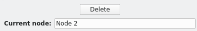
_images/processing_chain_node_selected.png

Simple change the name in the text field and press the Enter key on the keyboard to update the name in the model.

Source

The Source node is special and has its own edit settings. It defines what kind of model is being edited. By default it will have the following settings:

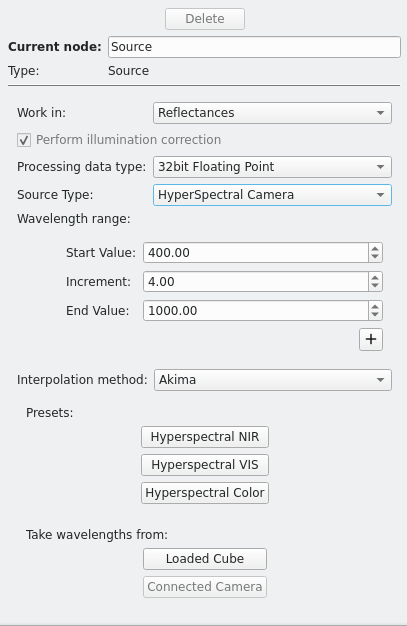
Work in

This settings defines the Value Type of the input data. This may be one of the following:

Reflectances: the data provided by the source will be reflectance values. Cubes that are loaded must be either in reflectances, or have a white reference present. See the Reflectance Measurements section in the concepts chapter for details.

Intensities: the data provided by the source will be intensities as they are returned by the sensor. This is incompatible with loading cubes that are available only as reflectances. If input data is provided in the form of Radiances or Relative Radiances (see below), that input data is considered to be compatible with the Source being set to this setting.

There are additional settings that are not shown by default, but can be enabled in the Data Viewer Options.

Absorbances: absorbances are defined as the negative decimal logarithm of the reflectances, i.e. $A = - \mathrm{log}_{10} R$ .

Radiances: radiance values are derived from sensor intensities by using calibration information to determine the absolute amount of light that has entered the detector. This will require that the input data must be provided as radiances (all other inputs will be rejected).

Relative Radiances: similar to Radiances, if the calibration only addresses some, but not all, of the physical effects relating the light entering the sensor to the intensity values. Setting the source to this setting will enforce that at least some correction has to have been performed on the input data. If the input data is provided in the form of absolute Radiances, that will also be compatible with the Source being set to this setting.

Perfrom illumination correction

If the Source is set to work in Intensities, Relative Radiances, or Radiances, this setting will ensure that an illumination correction is to be applied to the input data. This will require that the input data already had such a correction pre-applied when loading it, or that an illumination reference is present for the input data.

See the Illumination-Corrected Measurements section in the concepts chapter for details.

Processing data type

The user may select which floating point type to use to propagate the data throughout the graph. By default 32bit single-precision floating point values will be used (which is faster), but the user has the option to switch to 64bit double-precision floating point values. Using double-precision values is slower, but ensures a greater numerical stability for some algorithms.

Source Type

The user can select between two different types of camera:

HyperSpectral Camera: the source ensures that the input data has wavelengths aligned on a regular (equidistant) grid. See the Wavelength Abstraction section in the concepts chapter for details.

MultiSpectral Camera: the source will use exactly the wavelengths of a specific camera, not interpolating them at all. Input data is only compatible with the source if it has exactly the same wavelengths. This is most useful for analyzing images from cameras with very few spectral bands, where the distance between the bands is so large that interpolation does not make any sense, and models are specific to an individual camera anyway.

Selecting this is only possible if wavelengths have been imported from a specific loaded cube via e.g. the Loaded Cube button. (See below.)

Wavelength Range

In HyperSpectral Camera mode the user can specify the wavelength grid here. The grid consists of the following parameters:

Start Value: the lowest wavelength (in nanometers) of the grid

Increment: the spacing of the grid

End Value: the largest wavelength (in nanometers) of the grid

For example, with Start Value set to 400, Increment set to 4, and End Value set to 1000, there will be 151 values in the grid, namely 400 nm, 404 nm, 408 nm, …, 992 nm, 996 nm, 1000 nm.

It is also possible to define a sequence of grids by clicking on the plus button underneath the wavelength list. This is discussed in the advanced topics chapter in the Multiple Source Wavelength Grids section.

Note

When in MultiSpectral Camera mode the wavelength range edit is replaced by the list of wavelengths stored in the source. That list cannot be edited, it can only be replaced by using the Loaded Cube or Connected Camera buttons. (See below.)

Interpolation Method

In HyperSpectral Camera mode this allows the user to specify how the interpolation between the wavelengths should happen. The user may either select Akima, which will use the same algorithm as the Akima Interpolation Filter, or Linear, which will use the same algorithm as the Linear Interpolation Filter. The Akima method (the default) is more precise and better handles noise in the data, but is slower than a simple linear interpolation.

Presets

In HyperSpectral Camera mode these buttons allow the user to select from a list of sensible default ranges. There are three buttons:

Hyperspectral NIR: this will set the range to start at 950 nm, to end at 1650 nm, and to have an increment of 4 nm. It will mostly cover the range of typical InGaAs detectors. Those cover a range from 900 nm to 1700 nm, but in practice the data quality of most of these devices is very poor below 950 nm and above 1650 nm, which is why these are cut out by default.

Hyperspectral VIS: this will set the range to start at 400 nm, to end at 1000 nm, and to have an increment of 4 nm. It will cover the typical range of many silicon-based HSI cameras in the visible wavelength range.

Hyperspectral Color: this will set the range to start at 400 nm, to end at 800 nm, and to have an increment of 4 nm. It will cover the wavelength range of visible light that can be detected with a standard silicon-based HSI camera. This is the typical range for color measurements.

The default increment of 4 nm for all preset ranges is a good default across a multitude of HSI cameras, most of which have a full-width half-maximum close to that value.

Take wavelengths from

These buttons allow the user to automatically import the wavelengths from either a loaded cube or a connected camera.

The Loaded Cube button will only be enabled if all of the loaded cubes have the same exact wavelength values for their bands.

The Connected Camera button will only be enabled if a spectral instrument is currently connected.

In MultiSpectral mode the list of wavelengths will simply be copied and used as the exact wavelength list.

In HyperSpectral Camera mode it will set the start of the grid to the lowest wavelength of the list, the end of the grid to the highest wavelength of the list. The increment will be selected to be the smallest difference between two adjacent wavelengths in the list.

Note

When automatically taking the wavelength range from a camera or a cube, the resulting range will likely not be a very “nice” grid. It is therefore recommended to manually adjust the grid to be nicer, or to use one of the provided presets.

Filters and Sinks

The parameters of filters and sinks are shown in a generic tree, with the parameter names on the left side, and the method to edit the parameters on the right side.

Take, for example, the Distance Classifier Filter. It will have the following parameters:

_images/processing_chain_filter_parameters_distance_classifier.png

The filter gives a good overview over the possible types of parameters a node can have. On the top level the filter has 6 parameters:

Match Method, Distance Method, Base Quantity: these parameters are enumeration parameters, and have a drop-down to allow the user to select from a predefined list of options.

Threshold: this parameter is a floating-point parameter, i.e. the user specifies a number with a fractional part

KNN, Maximum Results: these parameters are integer parameters, i.e. the user specifies a number without a fractional part. Note also that the parameter KNN is disabled here, because whether it’s available or not depends on the value of other parameters

Then there is a category Output Configuration, which contains a single parameter:

Base Quantity: this is a boolean parameter, where the user can use a check box to switch the parameter on or off. In this case the parameter configures whether the filter has an additional output or not. This demonstrates how the number of inputs and outputs of a filter can be influenced by its parameters

Finally there is a single group-based parameter, Applicable. Group-based parameters are repeated for each group that is defined in the model and influence the filter on a per-group basis. The value set for one group may be different from the value set for another group. The most common group-based parameter across filters, Applicable, indicates whether a machine learning filter should take a specific group into account, or ignore it.