First Steps

In the following section it will be shown how to create a simple model with fluxTrainer that calculates absolute color values from HSI reflectance data. This will provide an introduction the basic functionality of fluxTrainer. In further sections the more advanced features of fluxTrainer will be explained.

Initial startup

When starting fluxTrainer for the first time, a message will appear that no license for fluxTrainer has been provided yet:

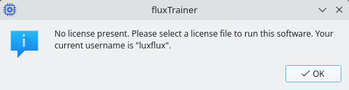
fluxTrainer always requires a license file. A license can be tied to various things, among them are:

The current mainboard

A disk/SSD in the current system

A hardware dongle

In the case of a hardware dongle, the dongle itself does not contain the license; instead it provides an id that the license file for fluxTrainer is tied to. The hardware dongle alone will not make fluxTrainer work.

Please contact sales@luxflux.de if you have not received your license file.

Once the message is acknowledged, a file selection window opens that requires the selection of the provided license file. fluxTrainer licenses always end in .lic.

If the license is accepted by fluxTrainer, it will start and show the main window. If there was an error regarding the license, a message will appear describing the issue, and fluxTrainer will ask for a license file again.

Pressing the Cancel button in the file selection window will exit fluxTrainer.

Once a license file has been accepted by fluxTrainer, its contents will be remembered. (The file itself does not matter anymore after it was read initially.) The next time fluxTrainer starts it will not ask for the license file again.

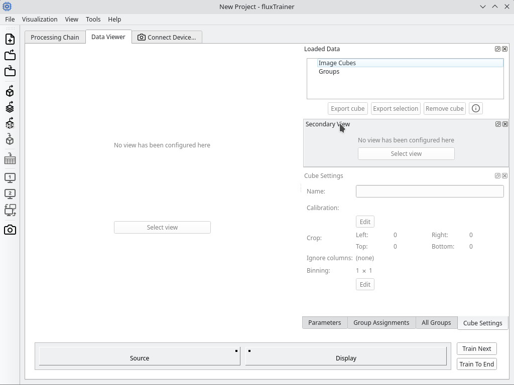
The main window of fluxTrainer will look like this after starting:

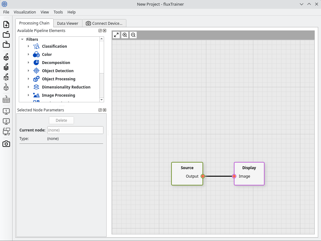
At the top there is a tab bar with tabs Processing Chain, Data Viewer, and Connect Device…. By default the Processing Chain tab will be selected.

Loading Data

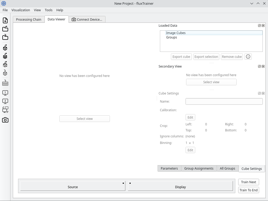
To load HSI cube data we first switch to the data viewer tab. This will show the following view:

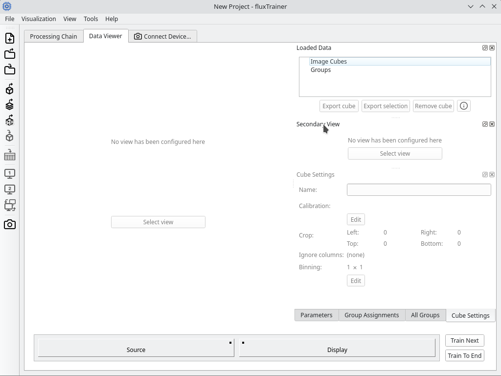
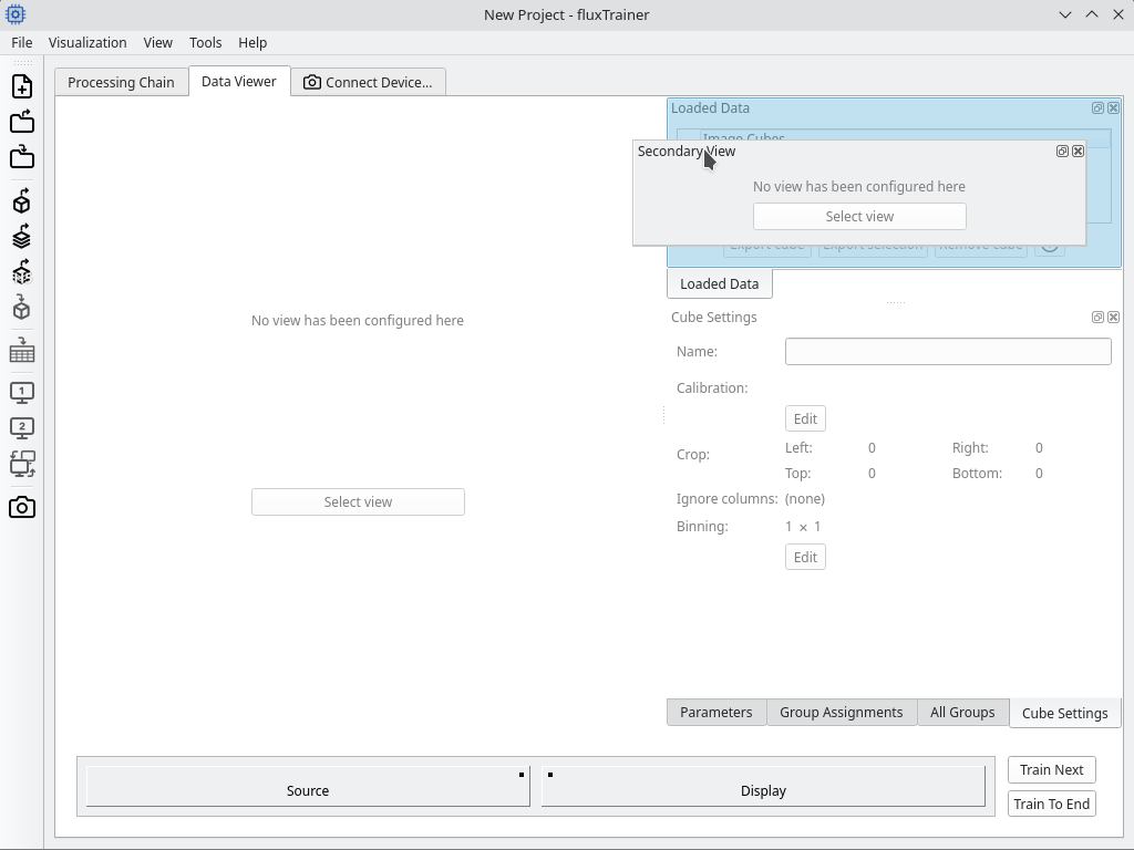
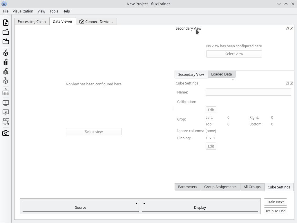
_images/first_steps_data_viewer_initial.png

To save a bit of screen real estate, we can now press the left mouse button on the secondary view and drag it on top of the loaded data dock widget:

_images/first_steps_data_viewer_drag_view2_1.png

_images/first_steps_data_viewer_drag_view2_2.png

_images/first_steps_data_viewer_drag_view2_3.png

_images/first_steps_data_viewer_drag_view2_4.png

We now load a HSI cube that is a recording of a color reference chart. To do so we click on the load cube button in the toolbar:

Alternatively we can also select the Import Data menu entry from the File menu.

This will open a file selection dialog. HSI cubes are typically stored in the ENVI format that is identified by a header file with the extension .hdr.

Note

HSI cubes are very large and hence use a lot of RAM.

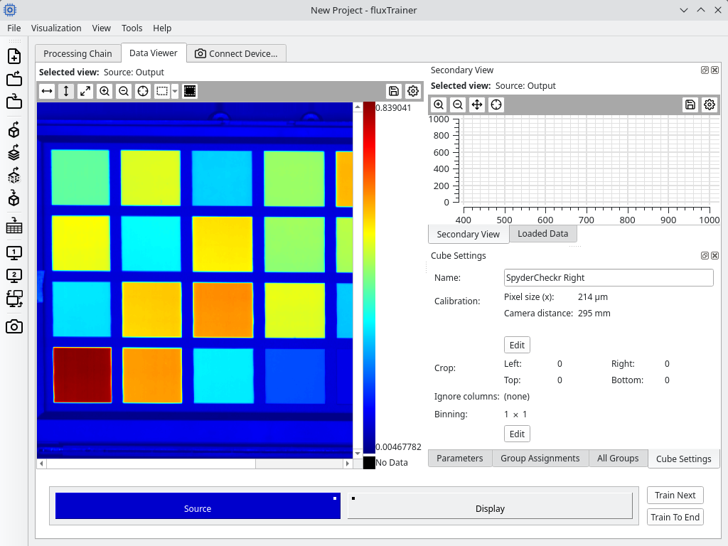
After selecting the appropriate HSI cube the data viewer will now display the loaded cube automatically:

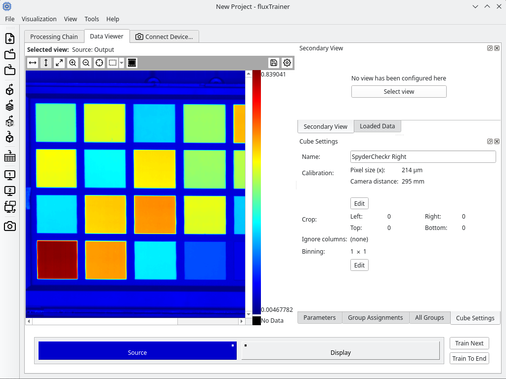
_images/first_steps_data_viewer_loaded.png

Here you can see the data viewer is separated into 5 areas:

On the left side there is a primary view

On the top right there is a list of loaded data and an empty area for the secondary view

On the bottom right there is a settings area with multiple tabs

At the very bottom there is an overview of all nodes in the model that can be stepped through to analyze the data

Image View

At first let us focus on the main image view. It will display an image of the loaded data. By default it will use a false-color image of the spectral average of the cube using a color map. A legend is displayed on the right hand side that shows the range of the color map. (By default the view will auto-range the color map based on the loaded data.)

Adding a spectral chart view

It is also possible to add a secondary view to further visualize the data that has been loaded. For example it might be interesting to see the raw spectra associated with the individual pixels. To add a secondary view, either click on the Select view button in the secondary view area (on the right hand side), or click on the Change Secondary View button in the toolbar:

_images/first_steps_secondary_view_toolbar.png

This will open a window where we can select the type of view to add:

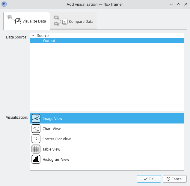
_images/first_steps_secondary_view_window_1.png

In this case we want to view the original spectra in addition to the image view. Select the Chart View:

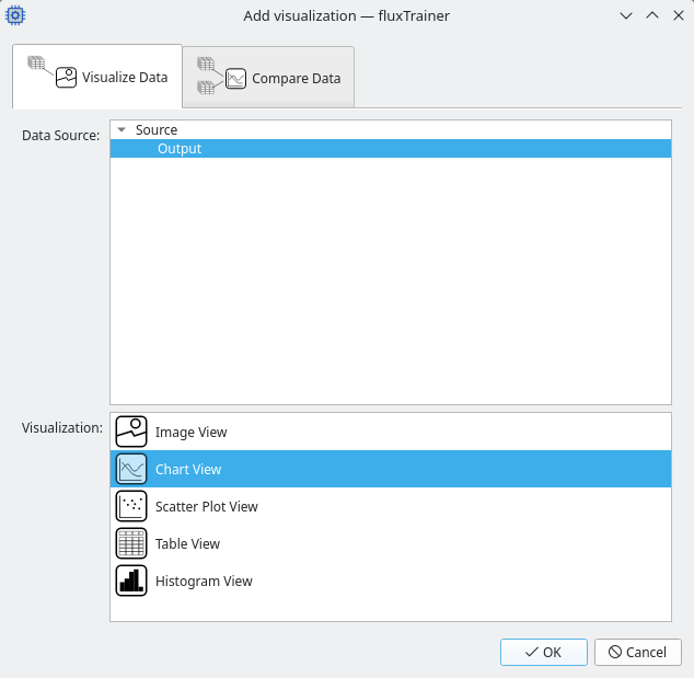
_images/first_steps_secondary_view_window_2.png

Replace the secondary view by clicking Ok. fluxTrainer will now display an empty chart view in addition to the spectra:

_images/first_steps_secondary_view_chart_empty.png

The spectral chart view is empty by default, because it will only show individual spectra that are currently selected. Selecting spectra can be done in the image view, using the selection tool:

_images/first_steps_secondary_view_pixel_selection_1.png

This will change the mouse cursor within the image view and the user can drag the mouse to select a rectangle:

_images/first_steps_secondary_view_pixel_selection_2.png

After releasing the mouse button the chart view will display the spectra that were selected by the user:

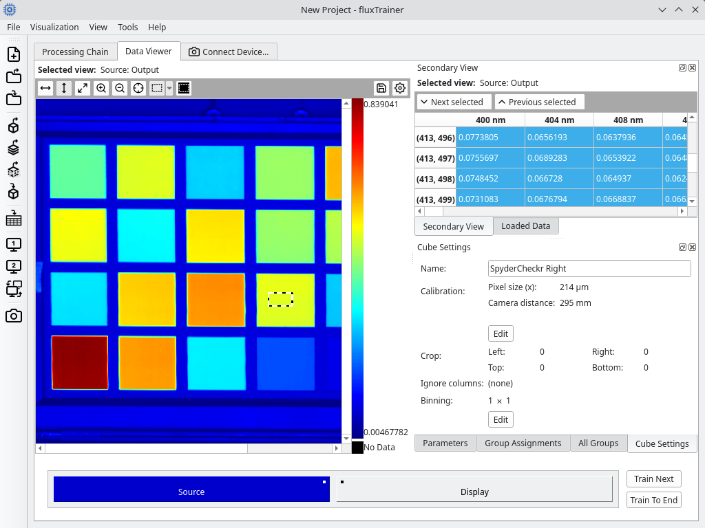
_images/first_steps_secondary_view_pixel_selection_3.png

Using a table view

Instead of a spectral chart view it is also possible to view the underlying values with a table view. For this we will replace the secondary chart view with a table view. Click on the Change Secondary View button in the toolbar again:

And then select a Table View to use as the view. This will replace the chart view with a table view that displays the individual reflectance values of the loaded data:

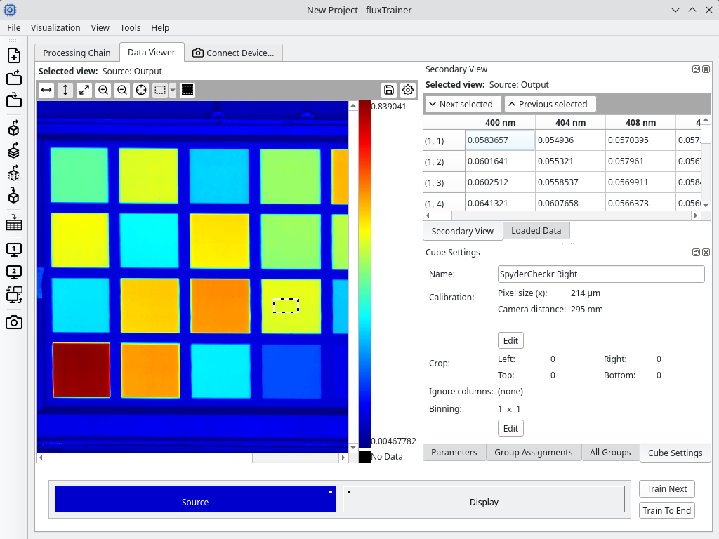
The rows of the table view denote the individual pixels. The pixels are shown as (y, x) in the table view, starting at (1, 1) in the display. For example, the pixel (30, 100) will be at y = 30 and x = 100. The columns are the channels that are available for each individual pixel. In this case the channels will be normalized spectral bands (that can be configured in the project’s source).

In a table view it is possible to jump to the next pixels that were selected by pressing the Next selected button. This allows us to quickly jump to the selected pixels and view the individual color values of those pixels:

Calculating Color Values

In the following example we want to calculate absolute color values for the given HSI cube. For this we need to switch back to the Processing Chain tab. There we can define the individual processing steps that will be applied to the data.

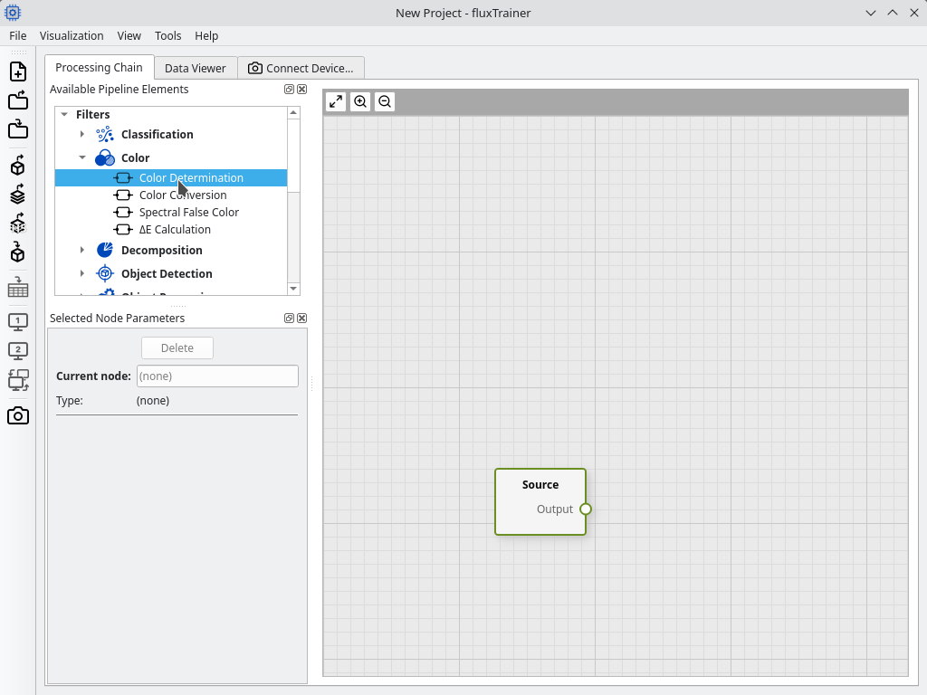
The Processing Chain tab of fluxTrainer consists of 3 main areas:

On the top left the user can see what nodes/filters are available to be added to the model.

On the bottom left the user can edit parameters of selected nodes.

On the right (the main area) the user can see the structure of the current model, and how data processing will happen. (This display is referred to as the Graph.)

We first remove the sink of the model.

Graph

The graph consists of nodes and connections between nodes. There are three main types of nodes:

Source: this is the node where the input data starts. It always has one output, the data that is to be processed. It has no inputs within the graph. Any data that is to be processed by the model starts at the Source.

Sink: a sink is a type of node that has one or more inputs, but no outputs. During data analysis in fluxTrainer itself, a sink will have no effect. But when using a model outside of fluxTrainer’s data analysis functionality (for example with fluxEngine), a sink will perform a specific operation with the input data it has been provided. This could be a visualization that is shown to the user, or it could be that data is written to disk. Sinks are optional, and for pure data analysis they are unnecessary.

Filter: a filter is any node that has both at least one input and at least one output. A filter applies an algorithm to the input data it is given. Filters provide the actual data processing functionality of fluxTrainer. There are a large variety of filters that perform a multitude of different tasks.

Inserting the color determination filter

At this stage we want to add the color determination filter that calculates the color value we desire. First we can delete the Display sink by right-clicking on it and selecting the Delete menu option:

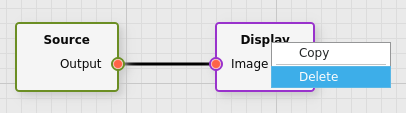
(Alternatively one can also left-click on the node to select it, and either press the Del key on the keyboard or click the Delete button above the node parameters.)

Now we can go to the list of filters, open the category Color, and select the filter Color Determination. Drag that filter from the list on the left hand side into the area with the graph, next to the Source:

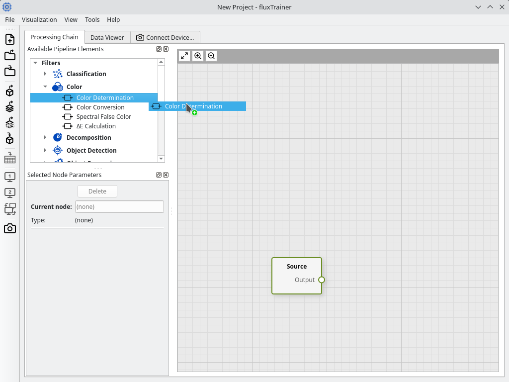
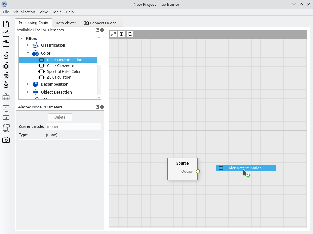
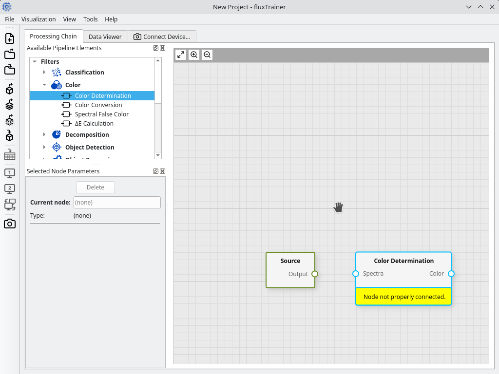
This will now create a new node in the graph for the Color Determination filter. The filter can be moved by dragging it across the background of the graph. This allows more complex models to be arranged so that they are more readable.

The new filter now needs to be connected. Drag the mouse from the output connection point on the source (the right side of the node) to the input connection point on the filter (the left side of the node):

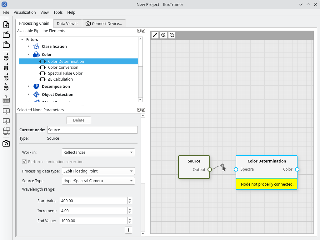
(It is also possible to disconnect nodes by dragging from the the input port of a node and dropping the connection anywhere in “free space”. Dragging from the output port of a node will always add a connection.)

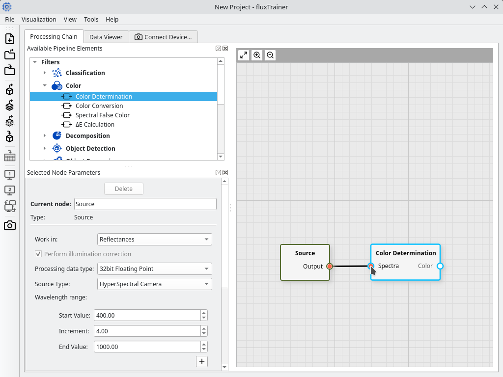
Now that the nodes are connected, click on the Color Determination filter to view its parameters:

All of the parameters that the filter supports are documented in the filter’s reference documentation, but in this case we want to change the color space to CIE L*a*b* color space:

_images/first_steps_filter_settings_changed.png

At this point we have created a basic model that can be used to calculate color values.

Visualizing The Color Values

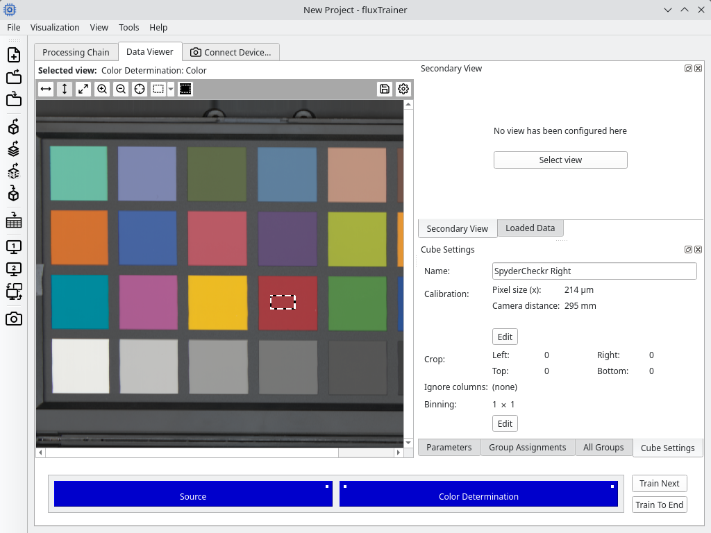
To visualize the color values we now switch back to the Data Viewer tab. There we will see that the bar at the bottom has changed and now contains the Color Determination filter:

_images/first_steps_data_viewer_with_filter.png

The bottom bar of the Data Viewer tab shows the nodes that are available in the model. Any node that has a blue backgroud is a node that has already performed the data processing during the current analysis. Any node that has a neutral background has not yet invoked its algorithm.

By selecting Train Next on the right hand side of the bottom bar fluxTrainer will process the input data with the next node in the model, and display those processing results:

_images/first_steps_data_viewer_train_next.png

In this case the user will see a different image view, namely that of the output of the color determination filter. Since fluxTrainer knows that the output of the color determination filter are color values, it will display those with actual colors to the user by default.

It should be noted that since this color image was reconstructed from HSI reflectance data, the color image is a measurement of the color chart that was calculated for an idealized reference illumination, not the actual illumination that was used to record the cube.

Saving the project

The project can now be saved. This can be done either via the save button in the toolbar:

Or by selecting the Save Project menu entry in the File menu. Both will open a file selection dialog that allows the user to specify a filename to save the project under.

A saved fluxTrainer project will have a .flux file extension and consists of both the model the user has created, as well as all of the loaded data.

The project can be loaded in fluxTrainer by selecting the load button in the toolbar (one above the save button), or the Load Project menu entry in the File menu. Alternatively, fluxTrainer registers the .flux file extension with the operating system in the installer, so a user should be able to open a fluxTrainer project directly from the operating system’s file manager.