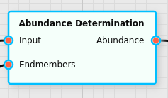
Abundance Determination Filter
Determines the abundnaces of input data with respect to a given list of endmembers.
Category |
|
Node |
|
Parameters |
InteractionType: determines the list of basis vectors for the abundances (see below) Constraints: which additional constraints to apply to the abundances. By default (Unconstrained) only a linear projection is done, which may cause some abundances to become negative. There are other constraints (see below) that perform an iterative algorithm to enforce certain mathematical properties. Iterations: the maximum number of iterations to perform when applying the constraints Output Configuration: allows the user to enable the optional outputs |
Inputs |
Input: the input data Endmembers: the endmembers to calculate the abundances for |
Outputs |
Abundance: the abundances Explained Spectra: the portion of the input spectrum that is explained by the abundances Error: the difference between the explained spectrum and the input spectra (this is also a spectrum) |
Effect of the Filter
The filter is generally used in combination with the Endmember Extraction Filter. It calculates the abundances for a given set of basis vectors.
The basis vectors are determined by the InteractionType parameter:
If InteractionType is SingleOnly, the basis vectors are just the endmembers that were provided via the second input of this filter
If InteractionType is DoubleOnly, the basis vectors are all pairwise coefficientwise products of all endmembers. For example, if three endmembers
,
and
were provided, then the basis vectors will be given by
,
, and
.
If InteractionType is SingleAndDouble, the basis vectors are the basis vectors of the SingleOnly case combined with the basis vectors of the DoubleOnly case. (For 2 endmembers this would mean 3 basis vectors; for 3 endmembers 6, for 4 endmembers 10, etc.)
The filter will attempt to represent the input data by a linear combination of the basis vectors, i.e.
where is the
-th abundance,
is
the error, and
is the input vector.
There are various constraints under which these coefficients can be determined:
In the Unconstrained case a simple projection onto the basis is performed (this is mathematically equivalent to performing an ordinary least squares fit). The abundances are then any real number.
The SumToOne constraint will cause the sum of the abundances to be equal to one (as best as numerically possible),
.
The Nonnegative and Semi-Nonnegative constraints will attempt to avoid negative values for the abundnaces, i.e.
, using two different matrix factorization algorithms in the iteration sequence.
